Introduction
Linear algebra is the backbone of Artificial Intelligence, from simple regressions to K-Means clustering. It's the essential toolkit AI employs to perform its wonders. Essentially, AI is a fusion of mathematics and computer processing. This blog delves into linear algebra concepts, offering insights into its crucial role. Subsequently, we'll delve into its integration within machine learning algorithms.
What are vectors?
Before we plunge into more intricate concepts, let's grasp the fundamental notion of a vector. Vectors can be categorized from three distinct viewpoints:
Physics
Computer science
Mathematics
Physics
In the realm of physics, a vector is visualized as an arrow extending through space, possessing both magnitude and direction. This concept encapsulates fundamental quantities like velocity, displacement, force, and acceleration. Vectors serve as a graphical representation to depict how objects move and interact in the physical world, enabling us to various physical phenomena.
Computer science
In the realm of computer science, a vector is akin to a list of numerical values that serve as a representation for datasets, particularly in the context of machine learning. In scenarios like image processing, each pixel can be treated as a matrix, contributing to the overall understanding of visual data.
$$\mathbf{v} = \begin{bmatrix} v_1 \\ v_2 \\ \vdots \\ v_n \end{bmatrix}$$
$$\mathbf{v} = \begin{bmatrix} v_1 = 1 \\ v_2 = 5 \\ v_3 = -2 \\ v_4 = 0 \end{bmatrix}$$
Mathematics
In the realm of mathematics, a vector is an arrow within a vector space, characterized by both direction and magnitude and emanating from the origin with its tail situated at the coordinates (0,0). This concept can be succinctly represented as follows:
$$\mathbf{v} = \begin{bmatrix} 2 \\ 3 \end{bmatrix}$$
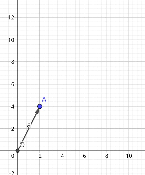
In this blog, our exclusive focus will be on the mathematical perspective of vectors.
What are Matrices?
A matrix is a rectangular array of numbers, symbols, or expressions arranged in rows and columns. It is a fundamental concept in linear algebra and is used to represent various types of data, such as transformations, systems of equations, and more. Matrices are commonly used to perform operations like addition, multiplication, and solving linear equations.
A matrix can be denoted as:
$$\begin{matrix} a & b & c \\ d & e & f \\ g & h & i \end{matrix}$$
Vector and Matrix Operations
Vector addition
Consider two 2-dimensional vectors, A and B. Vector addition involves calculating the sum of the individual x and y coordinates of these vectors. Graphically, this operation can be visualized by relocating the tail of vector B to the head of vector A. The resulting vector, known as the 'sum vector,' signifies the distance between the original tail of vector A and the new position of vector B. This graphical approach offers a tangible understanding of how vectors combine and yield a new direction and magnitude. The illustration will explain it further.
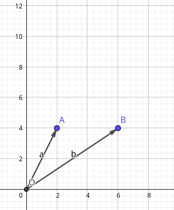
Vector A: Start by drawing vector A with its tail at the origin (0, 0) and its head at the point (2, 4).
Vector B: Draw vector B with its tail at the origin (0, 0) and its head at the point (6, 4).
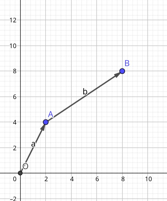
Move the vector B origin to the head of vector A
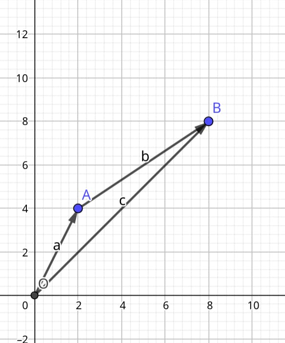
Now, connect the tail of vector A to the head of vector B. This resultant vector represents the sum of the two vectors.
In terms of Mathematics,
$$\vec{C} = \vec{A} + \vec{B}$$
$$\mathbf{A} = \begin{bmatrix} a_1 \\ a_2 \\ \end{bmatrix} \quad \text{and} \quad \mathbf{B} = \begin{bmatrix} b_1 \\ b_2 \\ \end{bmatrix}$$
$$\mathbf{C} = \mathbf{A} + \mathbf{B} = \begin{bmatrix} a_1 + b_1 \\ a_2 + b_2 \\ \end{bmatrix}$$
$$\mathbf{C} = \mathbf{A} + \mathbf{B} = \begin{bmatrix} 2 + 6 \\ 4 + 4 \\ \end{bmatrix}$$
$$\mathbf{C} = \mathbf{A} + \mathbf{B} = \begin{bmatrix} 8 \\ 8 \\ \end{bmatrix}$$
Matrix multiplication
Matrix multiplication can be imagined as a linear transformation in space. This transformation helps us understand where a set of vectors will end up when subjected to the transformation caused by other vectors. For a deeper grasp of this concept, I recommend watching 3blue1brown's video on Matrix multiplication. However, due to its complexity, a comprehensive explanation extends beyond the scope of a single blog.
Dot product
The dot product can be defined as the projection of one vector onto another. Let's consider two 2-dimensional vectors, A and B. The dot product is the sum of the products of the x and y coordinates.
$$\vec{A} \cdot \vec{B} = A_x \cdot B_x + A_y \cdot B_y$$
$$\vec{A} \cdot \vec{B} = \begin{bmatrix} A_x & A_y \end{bmatrix} \begin{bmatrix} B_x \\ B_y \end{bmatrix} = A_x \cdot B_x + A_y \cdot B_y$$
$$\vec{A} = \begin{bmatrix} 3 \\ -1 \end{bmatrix}, \quad \vec{B} = \begin{bmatrix} 2 \\ 4 \end{bmatrix} \vec{A} \cdot \vec{B} = \begin{bmatrix} 3 \\ -1 \end{bmatrix} \cdot \begin{bmatrix} 2 \\ 4 \end{bmatrix} = \begin{bmatrix} 3 & -1 \end{bmatrix} \begin{bmatrix} 2 \\ 4 \end{bmatrix} = (3 \cdot 2) + (-1 \cdot 4) = 6 - 4 = 2.$$
Types of Matrices
Matrices have various types based on their properties and characteristics. Here are some common types of matrices:
Square Matrix: A matrix where the number of rows is equal to the number of columns. It has the same number of rows and columns (n x n).
$$A = \begin{bmatrix} a_{11} & a_{12} & \dots & a_{1n} \\ a_{21} & a_{22} & \dots & a_{2n} \\ \vdots & \vdots & \ddots & \vdots \\ a_{n1} & a_{n2} & \dots & a_{nn} \end{bmatrix}$$
Rectangular Matrix: A matrix where the number of rows is not equal to the number of columns(m x n).
$$B = \begin{bmatrix} b_{11} & b_{12} & \dots & b_{1m} \\ b_{21} & b_{22} & \dots & b_{2m} \\ \vdots & \vdots & \ddots & \vdots \\ b_{n1} & b_{n2} & \dots & b_{nm} \end{bmatrix}$$
Zero Matrix: A square matrix where all diagonal elements are 1 and all other elements are 0. Denoted by 'I' or 'I_n', where 'n' represents the size of the matrix.
$$O = \begin{bmatrix} 0 & 0 & \dots & 0 \\ 0 & 0 & \dots & 0 \\ \vdots & \vdots & \ddots & \vdots \\ 0 & 0 & \dots & 0 \end{bmatrix}$$
Diagonal Matrix: A matrix in which all the non-diagonal elements are zeros. Diagonal matrices can be further categorized into scalar matrices (diagonal elements are all the same scalar) and diagonal matrices with distinct diagonal elements.
$$D = \begin{bmatrix} d_{11} & 0 & \dots & 0 \\ 0 & d_{22} & \dots & 0 \\ \vdots & \vdots & \ddots & \vdots \\ 0 & 0 & \dots & d_{nn} \end{bmatrix}$$
Upper Triangular Matrix: A square matrix where all the elements below the main diagonal are zero.
$$U = \begin{bmatrix} u_{11} & u_{12} & \dots & u_{1n} \\ 0 & u_{22} & \dots & u_{2n} \\ \vdots & \vdots & \ddots & \vdots \\ 0 & 0 & \dots & u_{nn} \end{bmatrix}$$
Lower Triangular Matrix: A square matrix where all the elements above the main diagonal are zero.
$$L = \begin{bmatrix} l_{11} & 0 & \dots & 0 \\ l_{21} & l_{22} & \dots & 0 \\ \vdots & \vdots & \ddots & \vdots \\ l_{n1} & l_{n2} & \dots & l_{nn} \end{bmatrix}$$
Symmetric Matrix: A square matrix that is equal to its transpose. In other words, the matrix remains unchanged when its rows and columns are swapped.
$$S = \begin{bmatrix} s_{11} & s_{12} & \dots & s_{1n} \\ s_{12} & s_{22} & \dots & s_{2n} \\ \vdots & \vdots & \ddots & \vdots \\ s_{1n} & s_{2n} & \dots & s_{nn} \end{bmatrix}$$
Skew-Symmetric Matrix: A square matrix that is equal to the negation of its transpose. This means that the elements below the main diagonal are negatives of the corresponding elements above the main diagonal.
$$A = \begin{bmatrix} 0 & a_{12} & a_{13} & \dots & a_{1n} \\ -a_{12} & 0 & a_{23} & \dots & a_{2n} \\ -a_{13} & -a_{23} & 0 & \dots & a_{3n} \\ \vdots & \vdots & \vdots & \ddots & \vdots \\ -a_{1n} & -a_{2n} & -a_{3n} & \dots & 0 \end{bmatrix}$$
Hermitian Matrix (Complex Symmetric Matrix): A matrix that is equal to its conjugate transpose (also known as Hermitian transpose or adjoint).
$$H = \begin{bmatrix} h_{11} & h_{12}^* & \dots & h_{1n}^* \\ h_{12} & h_{22} & \dots & h_{2n}^* \\ \vdots & \vdots & \ddots & \vdots \\ h_{1n} & h_{2n} & \dots & h_{nn} \end{bmatrix}$$
Unitary Matrix: A square matrix whose conjugate transpose is its inverse. In other words, the product of a unitary matrix and its conjugate transpose is the identity matrix.
$$U = \begin{bmatrix} u_{11} & u_{12} & \dots & u_{1n} \\ u_{21} & u_{22} & \dots & u_{2n} \\ \vdots & \vdots & \ddots & \vdots \\ u_{n1} & u_{n2} & \dots & u_{nn} \end{bmatrix}$$
Orthogonal Matrix: A square matrix whose transpose is its inverse. In the case of real matrices, this is equivalent to the matrix having orthogonal columns.
$$Q = \begin{bmatrix} q_{11} & q_{12} & \dots & q_{1n} \\ q_{21} & q_{22} & \dots & q_{2n} \\ \vdots & \vdots & \ddots & \vdots \\ q_{n1} & q_{n2} & \dots & q_{nn} \end{bmatrix}$$
These are just some of the many types of matrices that exist in mathematics. Each type has its significance and applications in various fields.
Conclusion
In the world of Artificial Intelligence, think of linear algebra as the secret ingredient that makes AI work. It's like the language AI uses to understand data and patterns, and make predictions. From simple things like arrows (vectors) that show directions, to grids of numbers (matrices) that help AI learn, linear algebra is what makes AI smart. So, if you're curious about how AI does its magic, understanding a bit of linear algebra is like having a superpower that lets you peek behind the curtain and see how the magic happens.
